[ArbLab] 2. TS Apprach (2) O-U Model Optimal Trading Thresholds Bertram/Zeng

 

페어 트레이딩 전략을 개발하기 위해 해결해야 할 두 가지 주요 문제는 1. 자산을 선택하여 평균 회귀 속성을 갖도록 하는 것과 2. 언제 거래할지를 결정하는 것이다. 두 번째 질문에 대한 일반적인 방법은 스프레드가 장기 평균에서 일정 금액 벗어날 때(ex historical standard deviation의 2~3배) 진입하는 것이다. 

 

이 포스트는 단위 시간당 기대 수익률을 최대화하는 것을 통해 진입 및 청산 threshold를 정하는 방법론에 대해 다룬다. 이 접근법은 Bertram (2010)에 의해 처음 논의되었고, 이후 Zeng 및 Lee(2014)는 초기 모델을 수정하여 롱 포지션 거래만 가능했던 제한을 제거했다.

임계값이 좁으면 거래를 완료하는 데 걸리는 시간이 짧지만 이익은 적다. 반면, 임계값이 넓으면 각 거래에서 얻는 이익은 크지만 거래를 완료하는 데 걸리는 시간이 길어진다. 즉 이익과 거래 시간 간의 최적화 문제이다. 가격이 Exponential Ornstein-Uhlenbeck 과정을 따르는 경우를 가정하고, first-passage time의 개념을 통해 trade length의 평균 및 분산을 도출하고, 단위 시간당 기대 수익과 수익 분산을 최대화하는 최적의 거래 임계값을 찾는다.

---

Assumptions

Price of the Traded Security

\[ p_t = e^{X_t} \]
여기서 \(X_t\)는 다음 확률 미분 방정식을 만족한다.
\[ dX_t = \mu(\theta - X_t)dt + \sigma dW_t \]

• \(\theta\)는 장기 평균
• \(\mu\)는 값이 장기 평균 주변으로 재조정되는 속도
• \(\sigma\)는 O-U 과정의 무작위성의 진폭

Trading Strategy

거래 전략은 \(X_t = a\)일 때 거래를 시작하고, \(X_t = m\)일 때 거래를 종료하는 것으로 정의된다.. 여기서 \(a < m\)이다.

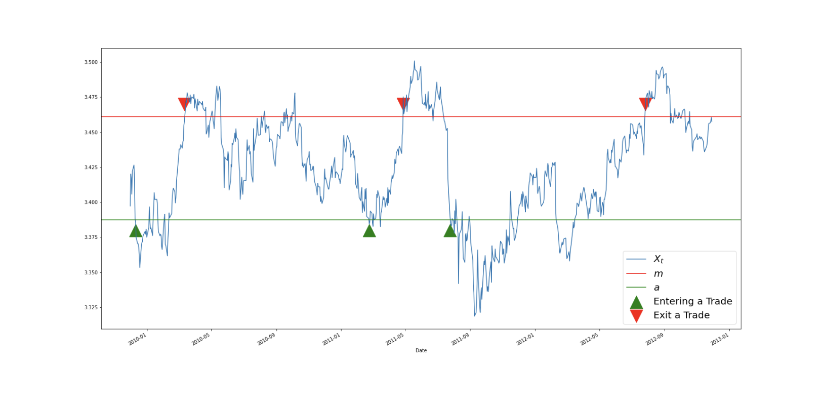
Trading Cycle

한 Cycle 은 \(X_t\)가 \(a\)에서 \(m\)으로, 다시 \(a\)로 돌아가는 것을 의미한다. 

 

Trading Length

Trading Leng \(T\)는  Trading Cycle를 완료하는 데 필요한 시간으로 정의한다.

 

이 두 개념은 자산 가격의 변동성과 거래 전략의 효율성을 분석하는 데 중요한 역할을 한다.  거래 사이클과 거래 길이를 통해 투자자는 시장에서의 거래 기회를 식별하고, 거래 전략의 성과를 평가할 수 있다.

---

Analytic Formulae

Mean and Variance of the Trade Length

a와 m을 어떻게 설정하냐에 따라 한 trading cycle의 시간이 달라짐 (단, m>a일 때만)

• a가 낮을수록, m이 높을수록 T가 길어짐
• a가 낮을수록, m이 높을수록 T의 분산이 커짐

\[ E[T] = \frac{\pi}{\mu} \left(\text{Erfi}\left(\frac{(m-\theta)\sqrt{\mu}}{\sigma}\right) - \text{Erfi}\left(\frac{(a-\theta)\sqrt{\mu}}{\sigma}\right)\right) \]
\[ V[T] = \frac{w_1\left(\frac{(m-\theta)\sqrt{2\mu}}{\sigma}\right) - w_1\left(\frac{(a-\theta)\sqrt{2\mu}}{\sigma}\right) - w_2\left(\frac{(m-\theta)\sqrt{2\mu}}{\sigma}\right) + w_2\left(\frac{(a-\theta)\sqrt{2\mu}}{\sigma}\right)}{\mu^2} \]
여기서 \(w_1(z)\)와 \(w_2(z)\)는 특정 함수이며, digamma 함수 \(\Psi(x)\)와 관련이 있다.

Mean and Variance of the Return per Unit of Time

\[ \mu_s(a, m, c) = \frac{r(a, m, c)}{E[T]} \]
\[ \sigma_s(a, m, c) = \frac{r(a, m, c)^2 V[T]}{E[T]^3} \]
여기서 \(r(a, m, c) = (m - a - c)\)는 거래의 연속 복합 수익률을 의미한다.

 

---

Optimal Strategies

Get Optimal Thresholds by Maximizing the Expected Return / Sharpe Ratio

최적의 거래 전략을 계산하기 위해, 기대 수익 또는 단위 시간당 샤프 비율을 최대화하는 최적의 진입 및 종료 임계값을 선택한다.

최대 기대 수익/샤프 비율은 \((m - \theta)^2 = (a - \theta)^2\)일 때 발생한다고 한다. 여기서 \(a < m\)을 가정하므로 \(m = 2\theta - a\)를 의미한다. 따라서 주어진 거래 비용/무위험 이자율에 대해 최적의 \(a\)와 \(m\)을 찾기 위해 다음 식을 최대화할 수 있다.

  \[
  \mu_s^*(a, c) = \frac{r(a, 2\theta a, c)}{E[T]}
\\
  S^*(a, c, r_f) = \frac{\mu_s(a, 2\theta a, c) - r^*}{\sigma_s(a, 2\theta a, c)}
  \]
  where \( r^* = \frac{r_f}{E[T]} \) and \( r_f \) is the risk-free rate

---

Implementation

Initializing OU-Process Parameters
O-U 과정을 초기화하는 방법에는 파라미터를 직접 설정하거나 주어진 데이터에 맞게 프로세스를 피팅하는 방법이 있다

Getting Optimal Thresholds
이 논문에서는 기대 수익과 샤프 비율이라는 두 가지 다른 목표 함수를 고려하여 최적의 전략을 선택하는 문제를 다룬다. 함수는 최적의 진입 임계값 \(a\)와 최적의 종료 임계값 \(m\)을 포함하는 튜플을 반환합니다.

Calculating Metrics and Plotting Comparison
최적의 임계값과 성능 지표를 사용하여 거래 전략의 성과를 계산하고 비교할 수 있습니다.

 

 

 

 

 

 

---

Assumptions

Price of the Traded Security

\[ p_t = e^{X_t}, \quad X_{t_0} = x_0  \]
  여기서 \( X_t \)는 다음의 확률 미분 방정식을 만족한다.
\[  dX_t = \mu (\theta - X_t) dt + \sigma dW_t  \]

•  \(\theta\): 장기 평균 (long-term mean)
• \(\mu\): 평균 회귀 속도 (mean-reversion speed)
• \(\sigma\): 무작위성의 크기 (amplitude of randomness)

Trading Strategy

  \[
  \begin{cases}
  \text{Y}_t = a_d 일 때 숏 포지션을 열고, \text{Y}_t = b_d 일 때 숏 포지션을 청산 \\
  \text{Y}_t = -a_d 일 때 롱 포지션을 열고, \text{Y}_t = -b_d 일 때 롱 포지션을 청산
  \end{cases}
  \]
여기서 \( Y_t \)는 원래의 시계열 \( X_t \)에서 변환된 무차원 시계열입니다. \( a_d \)와 \( b_d \)는 각각 무차원 시스템의 진입 및 청산 임계값이다
무차원 시계열(dimensionless series)은 단위가 없는 시계열 데이터를 의미한다. 이는 원래의 시계열 데이터를 변환하여 무차원화(dimensionless)하는 것을 말한다. 일반적으로 무차원화는 데이터를 특정 기준으로 나누거나 비례 변환을 통해 이루어진다.

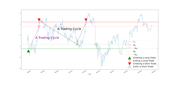
Trading Cycle

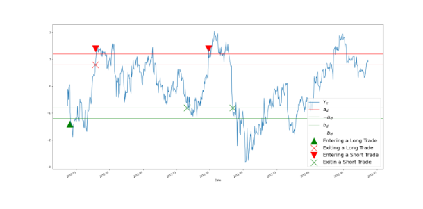
거래 사이클은 \( Y_t \)가 \( a_d \)에서 \( b_d \)로, 다시 \( a_d \) 또는 \(-a_d\)로 변할 때 완료된다

 \( a_d \)는 롱 포지션을 시작하거나 종료할 때의 가격 수준이고, \( b_d \)는 숏 포지션을 시작하거나 종료할 때의 가격 수준이다

Trade Length

거래 길이 \( T \)는 거래 사이클을 완료하는 데 필요한 시간으로 정의된다

예를 들어, 특정 주식의 가격이 \( a_d \) 수준에 도달하면 롱 포지션을 시작하고, \( b_d \) 수준에 도달하면 포지션을 종료한다. 이후 가격이 다시 \( a_d \) 수준으로 돌아오면 다시 롱 포지션을 시작하거나, \(-a_d\) 수준에 도달하면 숏 포지션을 시작하는 방식으로 거래 사이클이 반복된다. 이러한 방식으로 거래를 진행하면서 각 사이클의 길이 \( T \)를 측정하고 분석할 수 있다.

• 녹색 화살표: 롱 포지션 진입(Entering a Long Trade)
• 빨간색 화살표: 롱 포지션 종료(Exiting a Long Trade)
• 초록색 X: 숏 포지션 진입(Entering a Short Trade)
• 빨간색 X: 숏 포지션 종료(Exiting a Short Trade)

---

Analytic Formulae

Mean and Variance of the Trade Length

  \[
  E[T] = \frac{1}{2\mu} \sum_{k=0}^{\infty} \Gamma\left(2k + \frac{1}{2}\right) \left( (\sqrt{2a_d})^{2k+1} - (\sqrt{2b_d})^{2k+1} \right) / (2k + 1)!
\\
  V[T] = \frac{1}{\mu^2} (V[T_{a_d, b_d}] + V[T_{-a_d, a_d, b_d}]),
  \]

Mean and Variance of the Return per Unit of Time

단위 시간당 수익률의 평균 \( \mu_s(a, b, c) \)와 분산 \( \sigma_s(a, b, c) \)는 다음과 같다.
  \[
  \mu_s(a, b, c) = \frac{r(a, b, c)}{E[T]},
\\
  \sigma_s(a, b, c) = \frac{r(a, b, c) \cdot 2V[T]}{E[T]^3},
  \]
  여기서 \( r(a, b, c) \)는 거래 비용을 고려한 단일 거래의 연속 복리 수익률이다

Optimal Strategies

최적 거래 전략을 계산하기 위해, 주어진 거래 비용에 대해 단위 시간당 기대 수익률을 최대화하는 최적의 진입 및 종료 임계값을 선택한다.
- \( b_d = 0 \) 또는 \( b_d = -a_d \)일 때 최적 임계값을 찾기 위한 방정식을 해결합니다.
- 무차원 시스템에서 계산된 최적 임계값을 원래 시스템으로 변환하기 위한 공식:
  \[
  k = k_d \frac{\sigma}{\sqrt{2\mu}} + \theta,
  \]
  여기서 \( k_d = a_d, b_d, -a_d, -b_d \)입니다.

 

최적 거래 전략을 계산하기 위해, 주어진 거래 비용에 대해 단위 시간당 기대 수익률을 최대화하는 최적의 진입 및 종료 임계값을 선택합니다.

Get Optimal Thresholds by Maximizing the Expected Return

• Conventional Optimal Rule
  \(0 \leq b_d \leq a_d\)인 경우, \(b_d = 0\)일 때 최대 기대 수익률을 얻을 수 있다. 따라서, 주어진 거래 비용 \(c\)에 대해 다음 방정식을 해결하여 최적의 \(a_d\)를 찾는다.
  \[
  \frac{1}{2} \sum_{k=0}^{\infty} \Gamma\left(\frac{2k+1}{2}\right) \left( \sqrt{2a_d} \right)^{2k+1} / (2k+1)! = (a - c) \frac{\sqrt{2}}{2} \sum_{k=0}^{\infty} \Gamma\left(\frac{2k}{2}\right) \left( \sqrt{2a_d} \right)^{2k} / (2k+1)!
  \]
• New Optimal Rule
  \(-a_d \leq b_d \leq 0\)인 경우, \(b_d = -a_d\)일 때 최대 기대 수익률을 얻을 수 있다. 따라서, 주어진 거래 비용 \(c\)에 대해 다음 방정식을 해결하여 최적의 \(a_d\)를 찾는다. 
  \[
  \frac{1}{2} \sum_{k=0}^{\infty} \Gamma\left(\frac{2k+1}{2}\right) \left( \sqrt{2a_d} \right)^{2k+1} / (2k+1)! = (a - c \frac{\sqrt{2}}{2}) \sum_{k=0}^{\infty} \Gamma\left(\frac{2k}{2}\right) \left( \sqrt{2a_d} \right)^{2k} / (2k+1)!
  \]

 

Back Transform from the Dimensionless System

무차원 시스템에서 최적 임계값을 계산한 후, 이를 원래 시스템으로 변환하기 위해 다음 공식을 사용한다.
\[
k = k_d \frac{\sigma}{\sqrt{2\mu}} + \theta,
\\
\begin{cases}
k_d = a_d, b_d, -a_d, -b_d \\
k = a_s, b_s, a_l, b_l \\
\end{cases}
\]

\(a_s, b_s\)는 숏 포지션의 진입 및 종료 임계값을 나타내고, \(a_l, b_l\)는 롱 포지션의 진입 및 종료 임계값을 나타낸다

Implementation

Initializing OU-Process Parameters

OU-프로세스의 파라미터를 초기화하고 최적 임계값을 찾습니다. 초기 추정값(initial_guess)을 설정하여 계산 속도를 높인다

Calculating Metrics and Plotting Comparison

- 성능 메트릭 계산, 비교 플롯팅, 예제 코드 등을 통해 거래 전략의 성과를 분석한다

 

 

 

https://hudsonthames.org/optimal-trading-thresholds-for-the-o-u-process/

Optimal Trading Thresholds for the O-U Process - Hudson & Thames

https://hudson-and-thames-arbitragelab.readthedocs-hosted.com/en/latest/time_series_approach/ou_optimal_threshold_bertram.html

OU Model Optimal Trading Thresholds Bertram — arbitragelab 1.0.0 documentation

https://hudson-and-thames-arbitragelab.readthedocs-hosted.com/en/latest/time_series_approach/ou_optimal_threshold_zeng.html

OU Model Optimal Trading Thresholds Zeng — arbitragelab 1.0.0 documentation

https://hudsonthames.org/notebooks/arblab/ou_model_optimal_threshold_Bertram.html

ou_model_optimal_threshold_Bertram

https://hudsonthames.org/notebooks/arblab/ou_model_optimal_threshold_Zeng.html

ou_model_optimal_threshold_Zeng

https://www.youtube.com/watch?v=C7iZLMXyIOQ&t=337s